How to read this lesson
This is a guided reading of the 2017 paper "Attention Is All You Need" by Vaswani et al. The goal is not to memorize the Transformer diagram. The goal is to understand why each design choice exists, what math it uses, what problem it solved in 2017, and why the same ideas still appear inside modern language models, retrieval systems, coding models, multimodal models, and AI infrastructure.
We will move in the same order as the paper:
- The problem: sequence transduction was dominated by recurrent and convolutional models.
- The proposal: remove recurrence and convolution, and use attention as the main information-routing mechanism.
- The architecture: encoder stack, decoder stack, attention blocks, feed-forward blocks, residual connections, layer normalization, embeddings, and positional encodings.
- The math: scaled dot-product attention, multi-head attention, feed-forward networks, positional encodings, and the learning-rate schedule.
- The evidence: translation results, cost comparison, and ablation studies.
- The professional meaning: when Transformers help, where they are expensive, and what can go wrong in production systems.
Explain it in 5 minutes
The Transformer is a way to turn a sequence of tokens into useful contextual vectors without processing the sequence one step at a time. A contextual vectora vector whose meaning depends on the surrounding tokens, not just the current token alone. The word "bank" should have a different representation in "river bank" than in "bank account." Attention is the operation that makes that happen.
Here is the whole idea in one pass:
- Split text into tokens, then convert each token into an embedding vector.
- Add position information, because attention by itself does not know token order.
- For each token, create three learned views: a query, a key, and a value.
- Compare queries with keys to decide which tokens should exchange information.
- Use softmax to turn comparison scores into weights.
- Mix value vectors using those weights, producing a new contextual representation.
- Repeat this inside stacked encoder and decoder layers, with feed-forward networks, residual connections, and layer normalization keeping the computation expressive and trainable.
- In the decoder, hide future output tokens with a mask so generation cannot cheat.
The paper's breakthrough was not merely "attention exists." Earlier models already used attention. The breakthrough was showing that attention plus feed-forward layers could become the main sequence-processing backbone, replacing recurrence and convolution for the translation tasks studied in the paper. That made training more parallel, shortened the path between far-apart tokens, and achieved strong translation quality at much lower reported training cost than several prior systems.
If you only remember one tradeoff, remember this: full self-attention lets every token directly compare with every other token, but that creates an n by n attention score matrix. Direct communication is powerful; long context is expensive.
Learning objectives
By the end, you should be able to:
- Define sequence transduction, token, embedding, vector, hidden state, attention, self-attention, encoder, decoder, autoregressive generation, softmax, residual connection, layer normalization, dropout, and label smoothing.
- Explain why recurrent neural networks were slow to train on long sequences.
- Trace a token representation through the Transformer encoder and decoder.
- Compute the shape and meaning of
Q,K,V,QK^T,softmax, and the final value mixture. - Explain why dot products are scaled by
sqrt(d_k). - Explain why multi-head attention is not just "more attention," but parallel attention in different learned representation subspaces.
- Explain why positional encodings are needed when a model has no recurrence or convolution.
- Interpret the complexity table comparing self-attention, recurrence, and convolution.
- Read the training setup: data, batching, optimizer, warmup schedule, dropout, label smoothing, checkpoint averaging, beam search, and Bilingual Evaluation Understudy (BLEU).
- Connect the paper to modern professional systems: long-context cost, masking bugs, attention implementation efficiency, evaluation, and serving tradeoffs.
Prerequisites from zero
You do not need prior machine learning experience, but you need a few building blocks.
- A sequencean ordered list of items. A sentence is a sequence of words or word pieces. A generated answer is also a sequence.
- A sequence transductionthe task of turning one sequence into another sequence. Machine translation is the paper's main example: input is an English sentence, output is a German or French sentence.
- A tokena small unit a model processes. A token can be a word, part of a word, punctuation mark, or special symbol.
- A vectora list of numbers used to represent something. Neural networks operate on numbers, so text must become vectors before the model can compute with it.
- An embeddinga learned vector representation of a token. If a model learns useful embeddings, tokens used in similar ways often have related vectors.
- A matrixa rectangular table of numbers. A matrix lets the model process many vectors at once using optimized linear algebra.
- A parametera number learned during training. The model adjusts parameters so its predictions improve on training data.
- A probability distributiona set of nonnegative numbers that sum to 1. The model uses distributions to represent uncertainty over possible next tokens.
The paper assumes the reader already knows these ideas. This lesson will not.
Glossary of essential terms
| Term | Beginner definition | Professional meaning |
|---|---|---|
| Attention | A way for one token position to choose information from other positions. | The routing operation that compares queries with keys, then mixes values into contextual vectors. |
| Self-attention | Attention where the same sequence supplies the queries, keys, and values. | The core Transformer operation that lets all positions in a layer exchange information in parallel. |
| Query, key, value | Three learned views of a token representation: what it seeks, how it can be matched, and what it contributes. | The projected matrices Q, K, and V used in scaled dot-product attention. |
| Mask | A rule that hides positions the model should not use. | Essential for decoder training so a model cannot see future target tokens. |
| Residual connection | A shortcut that adds a layer's input back to its output. | A stability pattern that helps deep Transformer stacks preserve information and train reliably. |
| Positional encoding | Extra information that tells the model where each token appears. | The mechanism that gives an order-blind attention operation access to sequence order. |
The paper's central claim
Before the Transformer, strong sequence models usually combined an encodera network that reads the input sequence and produces useful internal representations. with a decodera network that produces the output sequence. The dominant encoder-decoder systems often used recurrent neural networks or convolutional neural networks, sometimes with an attention mechanism added on top.
The Transformer made a sharper claim: attention can be the core architecture, not just an add-on.
The title "Attention Is All You Need" means: for the translation tasks studied in the paper, the model can remove recurrence and convolution from the main sequence-processing path and rely on attention plus position-wise feed-forward networks.
- 1Input tokensText is split into model-readable pieces.
- 2Token embeddings + positional signalEach token becomes a vector, then position is added so order is visible.
- 3Encoder stackSelf-attention and feed-forward layers build contextual input vectors.
- 4Decoder stackMasked self-attention looks left; encoder attention looks back at the input.
- 5Next-token probabilitiesThe model scores possible next tokens and chooses or samples one.
That claim mattered because it changed the engineering profile of sequence modeling. Instead of processing one position after another, the model can compare all token positions in parallel inside each attention layer. This made training more efficient on graphics processing units (GPUs), which are very good at large matrix multiplications.
Paper reading map
| Paper section | What it contributes | What you should learn |
|---|---|---|
| Abstract and Introduction | The motivation: existing models were strong but sequential and slow. | Why parallelization and long-range dependency paths mattered. |
| Background | The comparison set: recurrent, convolutional, and earlier attention models. | What makes self-attention different from attention attached to a recurrent network. |
| Model Architecture | The encoder-decoder Transformer design. | How representations move through attention, feed-forward layers, residual paths, and normalization. |
| Why Self-Attention | The complexity argument. | Why self-attention has short paths but high long-sequence cost. |
| Training | The data, batching, optimizer, schedule, and regularization. | How the architecture was made trainable in practice. |
| Results and Variations | Translation scores, cost estimates, and ablations. | Which components mattered empirically and how the authors tested them. |
How the paper builds its argument section by section
Read the paper like an engineering argument, not like a list of components. Each section answers a different question.
Abstract and Introduction: what is the bottleneck?
The abstract makes three claims at once: the model removes recurrence, relies entirely on attention for global dependencies, and trains faster while reaching strong translation results. The introduction explains why this matters. Recurrent models create a sequential chain over positions, which limits parallel computation. Convolutional models parallelize better, but long-distance relationships require multiple layers or wider patterns.
Beginner move: whenever the paper says "dependencies," translate that into "one token needs information from another token." For example, a pronoun may need information from a noun many words earlier.
Background: what is actually new?
The background section prevents a common misreading. The authors did not invent every use of attention. Earlier encoder-decoder systems used attention, and other work explored convolutional sequence models. The new move was to make self-attention the main way information moves between positions in both the encoder and decoder.
Beginner move: separate "attention as a helper" from "attention as the backbone." The paper's claim depends on the second idea.
Model Architecture: how does the information flow?
This section is the blueprint. The encoder repeatedly applies self-attention and feed-forward layers. The decoder adds masked self-attention and encoder-decoder attention. Residual connections and layer normalization wrap every sub-layer so the model can be trained as a deep stack rather than as one fragile transformation.
Beginner move: do not try to memorize Figure 1 all at once. Trace one token through one sub-layer, then one encoder layer, then one decoder layer.
Attention: what is the exact operation?
The attention section turns the intuition into equations. A query-key dot product creates a compatibility score. Scaling keeps scores numerically manageable. Softmax turns scores into weights. The weighted sum of values creates the output. Multi-head attention repeats this in several learned subspaces.
Beginner move: read every matrix equation as a shape-and-meaning statement. Ask: What are the rows? What does each entry mean? What dimension must match?
Why Self-Attention: what tradeoff are the authors making?
This section is the professional heart of the paper. Self-attention has constant path length between positions and can be parallelized across positions inside a layer. The cost is the quadratic n^2 comparison matrix. The authors argue this is a good tradeoff for the sequence lengths and hardware setting they study.
Beginner move: do not confuse "parallel" with "free." Self-attention removes a sequential dependency, but it still performs many pairwise comparisons.
Training and Results: did the idea work under a real recipe?
The training section explains the system around the architecture: tokenization, batching, optimizer, learning-rate schedule, dropout, label smoothing, checkpoint averaging, and beam search. The results and ablations show both headline quality and sensitivity to design choices like head count, dimensions, dropout, and positional encoding type.
Beginner move: treat the result as architecture plus recipe plus evaluation setting. In professional work, a model is not just a diagram; it is also data, optimization, regularization, decoding, metrics, and hardware cost.
Section 1: Why recurrence was a bottleneck
The introduction starts from a practical problem. A recurrent neural networka network that processes a sequence step by step while carrying a hidden state forward. reads a sequence in order. For a sentence with positions 1, 2, 3, ..., n, the recurrent model computes one hidden state per position.
h_t = f(h_{t-1}, x_t)h_t is the hidden state at position t. A hidden state is the model's internal memory after reading up to that point. h_{t-1} is the previous hidden state. x_t is the input representation at the current position. f is the learned neural network function that combines the previous state with the current input.
The important dependency is h_t depends on h_{t-1}. That means the model cannot compute all positions at the same time within one example. It must wait for position 1 before position 2, and position 2 before position 3.
This creates two problems.
First, training is less parallel. GPUs are fastest when they can do many similar numerical operations at once. Sequential dependency limits that.
Second, long-distance relationships are hard. If a word near the end of a sentence depends on a word near the beginning, the signal may have to pass through many recurrent steps. Long paths can make learning unstable or inefficient.
Concrete example:
"The book that the students who studied late returned was expensive."
To understand "was," the model needs to know that the subject is "book," not "students." In a recurrent model, information about "book" has to survive several processing steps. In a Transformer self-attention layer, the representation at "was" can directly compare itself with "book" in one layer.
Section 2: What background problem the Transformer solves
The paper compares Transformers against three broad families:
- Recurrent models, which process tokens in a sequence of time steps.
- Convolutional models, which process local windows and need multiple layers or dilation to connect distant positions.
- Attention-augmented models, which already used attention but usually kept recurrence or convolution as the main backbone.
A convolutional neural networka network that applies the same local pattern detector across positions. can process positions in parallel, but a small convolution only sees nearby tokens. To connect far-apart tokens, the network needs more layers, wider kernels, or dilated patterns.
The Transformer uses self-attentionattention where queries, keys, and values all come from the same sequence. In the encoder, each input position can attend to every input position. In the decoder, each output position can attend to earlier output positions, and also to the encoder output.
The professional point is subtle: the paper is not just saying "attention works." It is saying attention can replace the sequential or local operation that previously moved information through the sequence.
Section 3: The encoder-decoder frame
Most translation systems in the paper's era used the same high-level frame:
- The encoder reads the source sentence.
- The encoder produces a sequence of continuous vector representations.
- The decoder produces the target sentence one token at a time.
- Each decoder step uses previous target tokens and information from the encoder.
The paper writes the input sequence as:
(x_1, ..., x_n)x_1 through x_n are the input symbols or token representations. n is the input sequence length. In translation, this might be the number of source-language tokens.
The encoder maps those inputs to:
z = (z_1, ..., z_n)z is the full sequence of encoder outputs. Each z_i is a vector representation for input position i after the encoder has mixed information across the sentence.
The decoder then generates:
(y_1, ..., y_m)y_1 through y_m are output symbols. m is the output sequence length. In translation, the output length can differ from the input length.
The decoder is autoregressiveit generates the next item using earlier generated items. If it is predicting token y_i, it can use y_1 through y_{i-1}, but it must not use future target tokens.
That is why masking exists. Masking is not decoration. It enforces the rule that generation cannot peek at the answer.
Section 3.1: Encoder stack from the paper
The original Transformer encoder has N = 6 identical layers. Each layer contains two sub-layers:
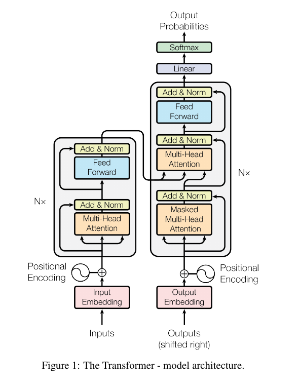
- Multi-head self-attention.
- A position-wise fully connected feed-forward network.
Every sub-layer is wrapped with a residual connection and layer normalization.
LayerNorm(x + Sublayer(x))x is the input vector or matrix entering the sub-layer. Sublayer(x) is the transformation performed by attention or the feed-forward network. The + adds the original input back to the transformed output. LayerNorm normalizes the result so activations stay in a more stable range.
A residual connectiona path that adds a layer's input to its output. helps information and gradients move through deep networks. Without residual paths, later layers can accidentally destroy useful earlier information or become harder to train.
Layer normalizationa normalization method that rescales features inside each example. helps keep the numerical values manageable as representations pass through many layers.
The paper sets d_model = 512 for the base model. This means the main representation width is 512 numbers per token position. The embedding layers and sub-layers all produce this same width so residual additions are shape-compatible.
Professional context: shape compatibility is a real implementation constraint. You cannot add two tensors unless their dimensions match or broadcast in a valid way. The paper's architecture keeps the main stream at d_model so residual connections are simple.
Section 3.2: Decoder stack from the paper
The decoder also has N = 6 layers, but each decoder layer has three sub-layers:
- Masked multi-head self-attention over the output tokens generated so far.
- Multi-head attention over the encoder output.
- A position-wise feed-forward network.
The first attention block is masked because the decoder must preserve autoregressive generation. During training, the correct output sentence is known, but the model must be trained as if it only knows earlier target tokens at each position.
Each output position may look at earlier target tokens, but future target tokens are hidden.
The second attention block is encoder-decoder attention. Its queries come from the decoder, while its keys and values come from the encoder output. In plain language, the decoder asks: "Given what I have generated so far, which source-language positions should I use now?"
Section 3.3: Attention from zero
Attention is a learned way to route information. One vector asks for information. Other vectors advertise what information they contain. The model computes match scores, turns those scores into weights, and uses the weights to mix content vectors.
The paper describes attention as mapping a query and key-value pairs to an output.
- A querya learned vector that represents what a position is looking for.
- A keya learned vector that represents what a position can be matched by.
- A valuea learned vector that represents the information contributed if that position is attended to.
- A compatibility functiona scoring rule that says how well a query matches a key.
Think about the sentence:
"The battery was old, so I replaced it."
At the token "it," a useful query might search for an object that can be replaced. The key for "battery" might match that query strongly. The value for "battery" then contributes information to the representation of "it."
This is not hard-coded. The model learns the projections that create queries, keys, and values during training.
Section 3.3.1: Scaled dot-product attention
The core equation is the heart of the paper.
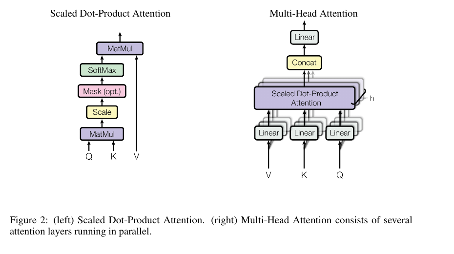
Attention(Q, K, V) = softmax((QK^T) / sqrt(d_k))VQ is the matrix of query vectors. K is the matrix of key vectors. V is the matrix of value vectors. K^T means the key matrix is transposed so every query can be compared with every key. d_k is the dimensionality of each key vector. sqrt(d_k) is the square root of that dimensionality. softmax turns scores into weights that sum to 1 across the keys. Multiplying by V uses those weights to mix the value vectors.
Break it into four operations.
Step 1: Compute match scores
Scores = QK^TEach entry in Scores compares one query with one key. If there are n tokens, this creates an n by n score matrix for self-attention. Row i says how much token i scores every token as a possible source of information.
A dot producta way to compare two vectors by multiplying matching components and summing the results.
q . k = q_1k_1 + q_2k_2 + ... + q_{d_k}k_{d_k}q is one query vector. k is one key vector. q_j is component j of the query. k_j is component j of the key. The result is one scalar score. A scalar is a single number.
If the dot product is high, the model treats the key as compatible with the query. If it is low, the model gives it less attention.
Step 2: Scale the scores
The paper divides by sqrt(d_k).
ScaledScores = (QK^T) / sqrt(d_k)d_k is the number of dimensions in each key and query vector. Dividing by sqrt(d_k) keeps the magnitude of scores from growing too large as the vectors get wider.
Why does this matter? Suppose each component of q and k behaves roughly like a random variable with mean 0 and variance 1. The dot product sums d_k products. The expected mean remains around 0, but the variance grows with d_k.
q . k = sum_{j=1}^{d_k} q_j k_j
Var(q . k) = d_k
sum means add across dimensions. Var means variance, a measure of how spread out values are. If the variance of the dot product grows with d_k, larger key dimensions can produce very large positive or negative scores.
Large scores make softmax too sharp.
Step 3: Apply softmax
softmax(s_i) = exp(s_i) / sum_j exp(s_j)s_i is one score in a row of attention scores. exp means the exponential function. sum_j exp(s_j) adds the exponentials of all scores in the same row. The output is a nonnegative weight. All weights in that row sum to 1.
Softmax turns raw scores into a probability-like distribution. If one score is much larger than the others, softmax can put almost all weight on one token. That may be useful sometimes, but if it happens too early or too often, gradients can become tiny for the ignored tokens.
A gradienta signal that tells training how to change parameters to reduce error. If gradients become extremely small, learning slows down.
Step 4: Mix values
Output = AttentionWeights VAttentionWeights is the matrix produced by softmax. V is the matrix of value vectors. Each output vector is a weighted average of value vectors.
This is the mechanism behind the phrase "a token attends to other tokens." More precisely: the token's query produces weights over keys, and those weights mix values into a new representation.
In scaled dot-product attention, what does `QK^T` produce?
A tiny numerical attention example
Imagine one query attends over three keys. After the model computes and scales dot products, suppose the scores are:
scores = [2.0, 1.0, -1.0]There are three possible source tokens. The first has the strongest match, the second is weaker, and the third is a poor match.
Softmax converts them into approximate weights:
softmax([2.0, 1.0, -1.0]) approx [0.705, 0.259, 0.035]The weights are nonnegative and sum to about 1. The first token contributes most, the second contributes some, and the third contributes very little.
If the three value vectors are v_1, v_2, and v_3, the output is:
output approx 0.705v_1 + 0.259v_2 + 0.035v_3The output is not a copied token. It is a new vector built from a weighted mixture of value vectors.
This matters in professional debugging. If attention weights are unexpectedly concentrated on irrelevant tokens, the output representation can carry the wrong evidence. In modern systems, this is one reason engineers inspect attention patterns, retrieved context, and model outputs together rather than trusting one visualization alone.
Implementation sketch: attention weights in code
This tiny example is not a production attention kernel. It is a beginner-sized way to connect the equation to executable steps: dot products, scaling, softmax, and weighted value mixing.
function dot(a: number[], b: number[]) {
  return a.reduce((sum, value, index) => sum + value * b[index], 0);
}

function softmax(scores: number[]) {
  const maxScore = Math.max(...scores);
  const expScores = scores.map((score) => Math.exp(score - maxScore));
  const total = expScores.reduce((sum, value) => sum + value, 0);
  return expScores.map((value) => value / total);
}

function weightedSum(weights: number[], values: number[][]) {
  return values[0].map((_, dimension) =>
    values.reduce((sum, value, index) => sum + weights[index] * value[dimension], 0)
  );
}

const query = [1, 0];
const keys = [
  [1, 0],
  [0.5, 0.5],
  [0, 1],
];
const values = [
  [10, 0],
  [4, 4],
  [0, 10],
];

const scaledScores = keys.map((key) => dot(query, key) / Math.sqrt(query.length));
const weights = softmax(scaledScores);
const output = weightedSum(weights, values);

console.log({ scaledScores, weights, output });
Professional note: real Transformer implementations batch this operation across examples, positions, heads, and layers. They also handle masks, padding, numerical precision, memory layout, and specialized kernels.
Section 3.3.2: Multi-head attention
One attention head gives one learned way to compare tokens. Multi-head attention gives several learned comparison spaces in parallel.
MultiHead(Q, K, V) = Concat(head_1, ..., head_h)W^O
head_i = Attention(QW_i^Q, KW_i^K, VW_i^V)
h is the number of heads. head_i is the output of attention head i. W_i^Q, W_i^K, and W_i^V are learned projection matrices for head i. W^O is the learned output projection after heads are concatenated. Concat means join the head outputs along the feature dimension.
In the base Transformer:
h = 8heads.d_model = 512.d_k = 64.d_v = 64.
The paper uses d_k = d_v = d_model / h, so each head is narrower than the full model width. Because there are eight heads of width 64, the combined width returns to 512 after concatenation.
Why not use one giant head? The paper's intuition is that a single attention operation averages information into one representation. Multiple heads let the model attend to different positions and representation subspaces at the same time.
Concrete language example:
- One head may attend from a pronoun to the noun it refers to.
- Another head may attend from a verb to its subject.
- Another may attend across punctuation or phrase boundaries.
- Another may track local neighboring tokens.
The paper does not claim heads are always cleanly interpretable, but it presents the possibility that attention patterns can expose some syntactic or semantic behavior.
Section 3.3.3: The three attention uses in the Transformer
The paper uses multi-head attention in three places.
1. Encoder self-attention
Queries, keys, and values all come from the previous encoder layer. Every input position can attend to every input position.
Professional meaning: this is how each input token becomes contextual. The representation of "bank" can change depending on whether nearby tokens mention money or rivers.
2. Decoder masked self-attention
Queries, keys, and values all come from the previous decoder layer, but future positions are masked.
masked_score = -infinity for future positions
softmax(masked_score) = 0
When a score is set to negative infinity before softmax, its softmax weight becomes 0. That prevents the decoder from using future output tokens.
Professional meaning: masking mistakes cause serious training and evaluation bugs. If future tokens leak into the decoder during training, the model may look excellent in training metrics while failing during real generation.
3. Encoder-decoder attention
Queries come from the decoder. Keys and values come from the encoder output. This lets each output position attend to the source sentence.
Professional meaning: this is the translation alignment mechanism. When generating a German word, the decoder can focus on relevant English source positions.
Section 3.4: Position-wise feed-forward networks
Attention lets positions communicate. The feed-forward network transforms each position independently after communication.
The paper's feed-forward equation is:
FFN(x) = max(0, xW_1 + b_1)W_2 + b_2x is the vector at one position. W_1 and W_2 are learned weight matrices. b_1 and b_2 are learned bias vectors. max(0, ...) is the Rectified Linear Unit (ReLU) activation, which replaces negative values with 0 and keeps positive values.
The same feed-forward network is applied to every position in a layer. "Position-wise" means the model does not mix information across positions in this sub-layer. Cross-token mixing happened in attention. The feed-forward layer performs per-token transformation.
In the base model:
- Input and output width:
d_model = 512. - Inner feed-forward width:
d_ff = 2048.
That means the feed-forward block expands each token vector from 512 dimensions to 2048 hidden dimensions, applies ReLU, then projects back to 512.
Professional context: in many modern Transformer variants, feed-forward blocks contain a large share of the model's parameters and compute. Attention is conceptually famous, but the feed-forward layers are also a major part of model capacity.
Section 3.5: Embeddings and output probabilities
The Transformer must convert discrete tokens into vectors.
Input side:
- Token IDs are looked up in an embedding table.
- The model gets one
d_model-dimensional vector per token. - Positional encoding is added.
- The result enters the encoder.
Output side:
- Previous output tokens are embedded.
- Positional encoding is added.
- The result enters the decoder.
- The decoder output is passed through a linear transformation.
- Softmax produces probabilities over possible next tokens.
The paper shares the same weight matrix between source embeddings, target embeddings, and the pre-softmax linear transformation, following earlier work. It also multiplies embedding weights by sqrt(d_model).
Why share weights? It reduces parameters and ties the input and output token representation spaces together. In language modeling and translation, the same vocabulary items often benefit from related input and output representations.
Section 3.6: Positional encoding
Self-attention alone has no built-in sense of order. If you give it the same token vectors in a different order, attention still compares token content, but the architecture itself does not know which token came first.
Compare:
- "dog bites person"
- "person bites dog"
The tokens are similar, but the meaning changes because the order changes. The model needs position information.
The paper adds positional encodings to the token embeddings at the bottom of the encoder and decoder stacks.
The sinusoidal positional encoding is:
PE(pos, 2i) = sin(pos / 10000^(2i / d_model))
PE(pos, 2i + 1) = cos(pos / 10000^(2i / d_model))
PE is the positional encoding. pos is the token position in the sequence. i is the dimension index. 2i refers to even dimensions. 2i + 1 refers to odd dimensions. d_model is the model width. sin and cos are sine and cosine functions.
Each position receives a pattern of sine and cosine values at different frequencies. Nearby positions have related patterns. Farther positions have different patterns. The paper chose this fixed sinusoidal approach partly because it might generalize to sequence lengths longer than those seen during training.
The authors also tested learned positional embeddings and found nearly identical results in their ablation table. That is important: the exact sinusoidal choice was not the only way to make the model work. The required idea is that position must enter somehow.
Professional context: modern Transformers use several positional strategies, including learned absolute positions, relative positions, rotary position embeddings, and attention biases. The same problem remains: attention needs order information.
Section 4: Why self-attention
The paper compares layer types using three criteria:
- Computational complexity per layer.
- How many sequential operations are required.
- Maximum path length between positions.
A path lengththe number of computational steps information must travel between two positions. Shorter paths can make it easier for the model to learn long-range dependencies.
The paper's complexity table can be read like this:
| Layer type | Complexity per layer | Sequential operations | Maximum path length |
|---|---|---|---|
| Self-attention | O(n^2 * d) | O(1) | O(1) |
| Recurrent | O(n * d^2) | O(n) | O(n) |
| Convolutional | O(k * n * d^2) | O(1) | O(log_k(n)) |
| Restricted self-attention | O(r * n * d) | O(1) | O(n / r) |
Symbol meanings:
nis sequence length.dis representation dimension.kis convolution kernel size.ris the neighborhood size for restricted self-attention.O(...)is Big O notation, a way to describe how cost grows as inputs grow.
Self-attention's major advantage is path length. Any token can directly connect to any other token in one attention layer, so maximum path length is O(1).
Self-attention's major cost is the n^2 term. Full attention compares every token with every other token. If sequence length doubles, the attention score matrix grows by about four times.
number_of_pairwise_scores = n * n = n^2If there are n query positions and n key positions, every query compares with every key. That creates n^2 scores per head before values are mixed.
This tradeoff still shapes AI infrastructure. Long-context models, retrieval-augmented generation, chunking, memory systems, and efficient attention kernels all exist partly because full attention over very long sequences is expensive.
What is the main long-context cost of full self-attention?
Section 5: Training data and batching
The paper evaluates on machine translation.
For English-to-German:
- Dataset: WMT 2014 English-German.
- Size: about 4.5 million sentence pairs.
- Tokenization: byte-pair encoding.
- Shared source-target vocabulary: about 37,000 tokens.
For English-to-French:
- Dataset: WMT 2014 English-French.
- Size: about 36 million sentence pairs.
- Tokenization: word-piece vocabulary.
- Vocabulary size: about 32,000 word pieces.
A byte-pair encodinga subword tokenization method that builds frequent character sequences into reusable token units. It helps handle rare words by breaking them into smaller known pieces.
A word piecea subword unit used to represent words as smaller reusable parts. For example, an uncommon word can be split into pieces the model has seen before.
The paper batches sentence pairs by approximate length. Each training batch contains about 25,000 source tokens and 25,000 target tokens. This matters because batching sequences of similar lengths reduces wasted padding.
paddingextra placeholder tokens added so sequences in the same batch have the same length. Too much padding wastes compute.
Professional context: batching strategy can affect training speed, memory use, and stability. In production inference, batching also affects latency and throughput.
Section 5.2: Hardware and schedule
The base models were trained on one machine with eight NVIDIA P100 GPUs. The paper reports:
- Base model: 100,000 steps, about 12 hours.
- Big model: 300,000 steps, about 3.5 days.
This was a central part of the paper's impact. The Transformer did not merely achieve strong translation quality; it did so with much less training cost than many competing systems in the comparison table.
Professional context: architecture quality is not only accuracy. Engineers also care about wall-clock training time, hardware cost, energy use, inference latency, memory footprint, and operational complexity.
Section 5.3: Optimizer and learning-rate schedule
The paper uses the Adam optimizer.
An optimizeran algorithm that updates model parameters during training. Adam is a popular optimizer that adapts update sizes using estimates of recent gradient behavior.
The paper uses:
beta_1 = 0.9beta_2 = 0.98epsilon = 10^-9warmup_steps = 4000
The learning-rate schedule is:
lrate = d_model^(-0.5) * min(step_num^(-0.5), step_num * warmup_steps^(-1.5))lrate is the learning rate, which controls update size. d_model is the model width. step_num is the current training step. warmup_steps is the number of initial steps where the learning rate increases. min(a, b) chooses the smaller of a and b.
This schedule does two things:
- During warmup, the learning rate increases roughly linearly.
- After warmup, the learning rate decreases in proportion to the inverse square root of the step number.
Why warm up? Early in training, parameters are not yet organized. A very large learning rate can destabilize training. Warmup lets the model start cautiously, then train more aggressively, then decay.
Professional context: learning-rate schedules are often as important as architecture details. A good architecture can fail with an unstable training recipe.
Section 5.4: Regularization
regularizationtechniques that reduce overfitting and improve generalization. Overfitting happens when a model performs well on training data but poorly on new data.
The paper uses three regularization ideas.
Residual dropout
dropouta training technique that randomly drops parts of a network's activations. This discourages the model from relying too heavily on any single path.
The base model uses dropout rate P_drop = 0.1.
Dropout on embeddings plus positional encodings
The paper also applies dropout after token embeddings and positional encodings are added. This regularizes the earliest representations entering the encoder and decoder stacks.
Label smoothing
label smoothinga training technique that makes the target distribution slightly less certain than a one-hot label.In ordinary classification, the target token might have probability 1.0, and every other token has probability 0.0. Label smoothing lowers the target probability a little and gives a small amount of probability mass to other tokens.
The paper uses epsilon_ls = 0.1.
Why do this? A model trained on perfectly sharp labels can become overconfident. Label smoothing can improve accuracy and BLEU even if it makes perplexity look worse.
perplexitya metric related to how surprised a model is by the correct tokens. Lower perplexity usually means the model assigns higher probability to the correct sequence, but label smoothing can complicate direct interpretation because the model is trained not to be perfectly certain.
Section 6: Results
The paper evaluates translation quality using Bilingual Evaluation Understudy (BLEU)an automatic metric that compares generated translations with reference translations using overlapping word or subword patterns.
BLEU is not a perfect measure of translation quality. It can miss meaning, fluency, and acceptable paraphrases. But it was a standard benchmark metric for machine translation, so it allowed the authors to compare with prior systems.
The headline results:
- On WMT 2014 English-to-German, the big Transformer achieved 28.4 BLEU.
- On WMT 2014 English-to-French, the big Transformer achieved 41.0 BLEU in the paper body, and the abstract reports a 41.8 BLEU single-model headline result after checkpoint averaging.
- The base Transformer already surpassed many earlier published systems at lower estimated training cost.
- The big Transformer beat prior single-model systems on English-to-French with less than one quarter of the training cost of the previous state-of-the-art model cited in the paper.
The paper also uses checkpoint averaging and beam search.
checkpoint averagingcombining several saved model checkpoints to get a more stable final model. beam searcha decoding algorithm that keeps several likely partial output sequences at each generation step instead of only the single best next token.The paper used beam size 4 and length penalty alpha = 0.6. A length penalty adjusts the score so the decoder does not unfairly prefer overly short or overly long translations.
Professional context: evaluation results depend on training recipe and inference recipe. When comparing models, engineers need to ask: What data? What tokenization? What checkpoint selection? What decoding settings? What metric? What hardware cost?
Section 6.2: Model variations and ablations
An ablation studyan experiment that changes or removes parts of a system to see what matters. Ablations are how papers move from "this worked" to "these parts seem important."
The paper varies several components.
Number of heads
The base model uses 8 heads. The ablation table shows that 1 head performs worse. Too many heads can also hurt when each head becomes very narrow.
Interpretation: multiple heads help, but not infinitely. There is a tradeoff between number of heads and dimension per head.
Key and value dimensions
Reducing key size hurts quality. The paper suggests that compatibility between queries and keys is not trivial. The model needs enough representational room to decide what should attend to what.
Model size
Bigger models generally perform better in the table. The big model uses:
d_model = 1024d_ff = 4096h = 16- about 213 million parameters
The base model has about 65 million parameters.
parameter countthe number of learned numbers in a model. More parameters often increase capacity, but they also increase memory use, compute cost, and overfitting risk.
Dropout
The ablations show dropout is helpful for avoiding overfitting. This is a reminder that architecture alone is not enough. The regularization recipe matters.
Positional encodings
Replacing sinusoidal positional encodings with learned positional embeddings produced nearly identical results in the reported ablation. This supports the idea that position information is necessary, while the exact method can vary.
What the paper did not solve
The Transformer was a breakthrough, not a final answer.
It did not eliminate sequential generation. The decoder still generates output tokens autoregressively, one position at a time, because token y_i depends on earlier generated tokens.
It did not make long context free. Full self-attention has O(n^2) attention scores. Long documents, audio, video, and high-resolution images can make this expensive.
It did not prove attention weights are always faithful explanations. Attention patterns can be informative, but a model's behavior is distributed across embeddings, projections, feed-forward layers, normalization, and decoding.
It did not address all production evaluation issues. BLEU is useful for machine translation benchmarking, but production systems need task-specific evaluation, human review, robustness testing, latency measurement, cost tracking, and failure analysis.
Common misconceptions
Misconception: "Attention is memory."
Better view: attention is information routing over vectors available in the current computation. It can retrieve information from the current context, but it is not the same as a persistent database or long-term memory system.
Misconception: "The Transformer has no order."
Better view: raw self-attention is order-blind, so the architecture injects order through positional encodings or related mechanisms.
Misconception: "Multi-head attention means heads manually represent grammar rules."
Better view: heads are learned projections. Some heads may show interpretable patterns, but the model is not guaranteed to allocate one clean linguistic function per head.
Misconception: "The paper is only about large language models."
Better view: the paper studied machine translation. Later large language models adapted Transformer ideas, especially decoder-only autoregressive variants, at much larger scale and on broader data.
Misconception: "Transformers are always better than recurrent or convolutional models."
Better view: Transformers are extremely powerful, but architecture choice depends on data size, sequence length, latency constraints, hardware, inductive bias, and deployment setting.
Production failure modes to watch for
- Masking bugs: the decoder or language model sees future tokens during training or evaluation.
- Shape bugs:
Q,K,V, head dimensions, batch dimensions, or residual dimensions do not line up. - Position bugs: positional encodings are missing, misaligned, truncated, or inconsistent between training and inference.
- Padding bugs: attention attends to padding tokens because padding masks are wrong.
- Long-context cost surprises: memory or latency grows sharply as sequence length increases.
- Evaluation mismatch: the benchmark metric improves, but the user-facing task does not.
- Overconfidence: the model assigns high confidence to wrong outputs, especially when regularization or calibration is weak.
- Source confusion in retrieval systems: the model attends over irrelevant or low-quality context and produces fluent but unsupported answers.
Professional engineers do not just ask whether attention works. They ask whether the attention implementation is correct, efficient, masked properly, evaluated honestly, and serving within cost and latency limits.
Interview-ready summary
A Transformer turns tokens into vectors, adds position information, and repeatedly applies attention plus feed-forward transformations. In self-attention, each position creates a query, key, and value. Queries compare with keys through scaled dot products. Softmax turns those scores into weights. The weights mix values into new contextual representations. Multi-head attention performs this process several times in parallel in different learned projection spaces. Encoder layers use self-attention over the input. Decoder layers use masked self-attention over previous outputs and encoder-decoder attention over the source sequence. The architecture trains efficiently because positions in a layer can be processed in parallel, but full attention is expensive for long sequences because it compares every token with every other token.
Practice: trace one token through the encoder
Use the sentence:
"The animal did not cross the street because it was tired."
Trace the token "it."
- Tokenization turns the text into token IDs.
- The token ID for "it" becomes an embedding vector.
- A positional encoding is added so the model knows where "it" appears.
- In encoder self-attention, the "it" query compares with keys from all input positions.
- Tokens such as "animal" may receive high attention weights if useful for resolving reference.
- The weighted value mixture updates the representation of "it."
- The feed-forward network transforms the updated representation at that position.
- Residual connections preserve earlier information, and layer normalization stabilizes the representation.
- Repeating this across layers builds a richer contextual vector.
Which statement best describes the encoder's output?
Practice: reason about costs
Suppose a self-attention layer processes n = 1,000 tokens. One head creates about:
n^2 = 1000^2 = 1,000,000 scoresThis is only the attention score matrix for one layer and one head, before considering batches, multiple heads, value mixing, feed-forward layers, or backpropagation during training.
If n = 2,000, then:
n^2 = 2000^2 = 4,000,000 scoresDoubling the sequence length quadruples the number of pairwise scores.
This is why long context is an infrastructure problem, not just a modeling feature.
Final mastery checklist
You should not need to read the paper separately to understand its main argument. Use this checklist to confirm that the lesson gave you the same core understanding in a more beginner-friendly path:
- Explain the paper's claims about translation quality, parallelization, and training time.
- Describe the sequential bottleneck that made recurrent models harder to parallelize.
- Trace the residual-plus-normalization pattern around every Transformer sub-layer.
- Write the scaled dot-product attention equation and label every symbol.
- Explain how eight attention heads of width 64 relate to
d_model = 512. - Explain why positional information must be added when recurrence and convolution are removed.
- Distinguish path length from computational complexity.
- Separate the architecture choices from the training recipe.
- Use the ablation results to identify which design choices seem robust and which seem sensitive.
You are ready for the next lesson when...
- You can explain why self-attention lets each token gather information from other tokens in the same sequence.
- You can describe how queries, keys, values, softmax weights, and value mixing work together.
- You can explain why positional information is necessary in a Transformer.
- You can identify the main production risks: masking bugs, padding bugs, shape bugs, and long-context cost.
- You can connect the original translation paper to modern language models without treating them as the same system.